Sensors - Synchronous Detection - Part II - EdsCave
Main menu
- Home Page
- Sensors
- Simulation
- Analytics
- Forecasting
- Football Forecasting
- Random Corner
- Projects
- Resources
- Blog
- About/Contact
- Creative Works
- Separator 1
- Privacy & Terms
Sensors - Synchronous Detection - Part II
9 May 2016
How Synchronous Detection Works
In Part 1 of this blog, we introduced the synchronous detection technique as a way to reduce noise in sensing systems. In this installment we will discuss how synchronous detection actually performs its noise-
In this system, the transducer multiplies its true measured signal by the modulation signal, or carrier. To do this means that the sensitivity or 'gain' of the sensor is somehow varied by the carrier. For bridge-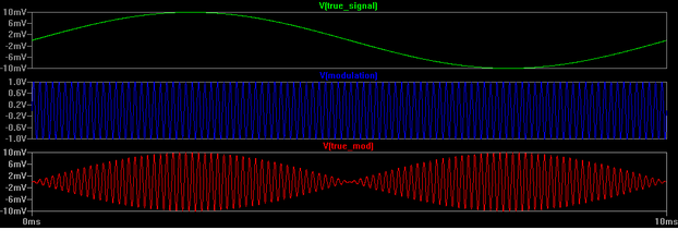
Recovering the transducer signal is the reverse process, with post-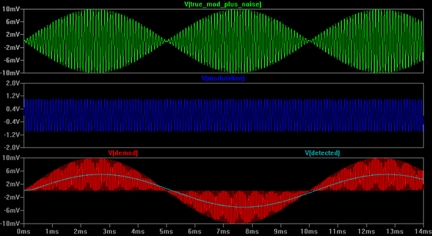
The power of synchrounous detection becomes apparent when we apply the demodulation/filter process to something that isn't the modulated transducer signal. In the plots below, the top trace (green) shows an interfering signal comprising both white noise and sinusoidal interference. In this case, there is no modulated transducer signal present. The sinusoidal interference is set to a frequency (60 Hz) not all that different from that of the transducer signal shown above (100Hz). Because the two frequencies are so close together, trying to remove this interference by filtering would require a fairly sophisticated filter. Note, however, what happens when the interfering signal is demodulated. Because it is not synchronized with the modulating signal, it ends up being 'chopped' into a roughly equal number of positive and negative parts at the modulating frequency (red-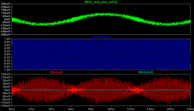
The demodulation and filtering process is very similar to finding the statistical covariance between the modulated transducer signal and the carrier. The only signals that would be expected to have a high covariance (either postive or negative) with the carrier are those that have very similar frequency and phase characteristics. Using a carrier with significantly higher frequency than that of the transducer signal allows one to effectively take more 'samples' for the covariance (longer filtering time) so as to get more significant results.
Another way to understand how synchronous detection works is through its frequency-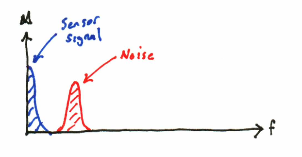
The effect of modulating the sensor signal is to shift it upward in frequency by the carrier frequency (Fmod -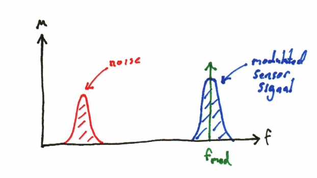
Now if we demodulate the above spectrum using the same carrier frequency, several things happen:
The previously modulated transducer signal is shifted back down so that it at DC. Additionally, (but not shown), a copy of the transducer spectrum is created that is centered at 2 x Fmod (twice the modulation frequency).
The noise signal is upshifted by Fmod. Also, a second copy is created that is symmetrically mirrored around Fmod, but on the lower side.

If Fmod is significantly higher that the transducer signals, then it shifts any interference in proximity to the transducer signals far away from the transducer signals. Since it has been moved away from the transducer signals, the interference can then be easily filtered out.
But what about the case where the interference is close to the carrier frequency? This does pose a problem. If the interference is at the same frequency and phase as the modulation signal, it will be detected along with the signal. One big advantage of synchronous detection is that within wide limits, you get to pick your modulating frequency. For example, in the US 60Hz is the standard power-
In the final part of this blog we will discuss some techniques for practical implementation.