Forecasting - Metrics for Time Series Forecasts - EdsCave
Main menu
- Home Page
- Sensors
- Simulation
- Analytics
- Forecasting
- Football Forecasting
- Random Corner
- Projects
- Resources
- Blog
- About/Contact
- Creative Works
- Separator 1
- Privacy & Terms
Forecasting - Metrics for Time Series Forecasts
If you're engaged in the task of making time-
A time-
Defining Error
The fundamental core of any evaluation technique is the definition of deviation from the ideal or error. For the purposes of comparing our forecasts to reality, we will define error as the difference between the actual value for a given actual datum in the time series (Ai) and the forecast value (Fi):
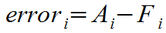
The order of the subtraction in this definition of error may be a little counter-
Absolute Error Metrics
While being able to quantify the error for each data point is important, basing an evaluation off a single data point is neither particular wise nor useful. Because the actual data will typically contain some 'random' variation (or at least poorly understood variation) and some of that noise will find its way into any forecast based on it, some portion of the Actual-
Consider the hypothetical monthly forecast and actual sales for ChocoNuclear Crunch, shown in the table below. The actual figures are what would be counted shipping from the factory at the end of each month, while the forecast figures would normally be developed before this time, when the actual were not known. It is for this reason that while there is a forecast figure for October, the 'actual' figure is labeled TBD, because the month's data is not available. The final line in the table is the 'Ai – Fi' error for each month.

The first metric we will look at is the Mean Error (ME), which is simply the average of all the individual errors and given by the formula below.
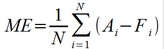
Mean Error measures a forecast's bias, which is one type of error. If your forecasts are consistently low, the ME metric will be positive, while if they run consistently high, the ME metric will be negative. When applied to the above table of ChocoNuclear Crunch sales, this metric yields 166.7, indicating that the average forecast is biased a little lower than the actual shipments. Interestingly, if you were to have a forecast where some individual errors were positive, and others negative, the overall ME could equal zero even with a set of forecasts that widely diverged from actual. For this reason, while ME can indicate systematic bias (valuable information), it is not useful as a measure of how 'good' the forecast is.
In statistics, it is very common to 'square' error terms. This avoids the pitfall where positive and negative errors can cancel each other out (as was the case with ME), as a squaring operation makes all error terms positive. This same technique can be readily applied to time-
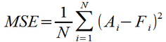
One drawback of the squaring operation makes the magnitude of MSE not directly comparable to that of the original errors – for example, the MSE for the ChocoNuclear Crunch forecast is 1,083,333, which is difficult to relate to the magnitudes of the monthly shipments. One solution is to take the square root, yielding the metric Root-

The RMSE metric for ChocoNuclear Crunch yields 1040, which is of comparable magnitude to the individual monthly errors. With MSE, as with the other metrics to be described in this article, a lower value indicates a better forecast. One property of the RMSE metric is that it more heavily penalizes larger errors due to the squaring operation. For example, an error of '2' in a given month carries as much weight as an error of '1' in four separate months combined. This feature has both advantages and disadvantages. On the positive side, it means that the RMSE metric will favor a forecasting technique in which the individual errors tend to be of consistent magnitude, as wide variations in error will tend to drive the RMSE metric higher. The disadvantage is the flip side of this – a few bad forecast points in an otherwise very good forecast can drive up the RMSE figure, masking otherwise good performance.
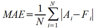
One way to minimize the effects of a few 'outlier' bad forecast points is to switch from squaring the error to taking the absolute value. In the Mean Absolute Error (MAE) metric shown below, large errors only have a proportional effect on the overall metric. An error of '2' makes the same contribution as two errors of '1'.
Relative Error Metrics
While the absolute error metrics presented above are fine for comparing the effectiveness of different forecasting techniques when applied to the same time series, they are less useful when comparing effectiveness across multiple time-
One way to make a metric that is useful for comparing forecasts on disparate-
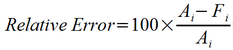

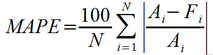
The relative error then may be substituted for the error terms in the metrics described above. The most commonly encountered relative error metrics are Mean Percentage Error (MPE), and Mean Absolute Percentage Error (MAPE). For the above forecast, MPE = 0.98%, while MAPE = 8.09%. As was the case for ME, MPE is a metric for high or low bias, while MAPE is useful as an overall accuracy. The formulas for MEA and MAPE are shown below.

While it is possible to develop a Root-
Unlike the absolute error metrics initially presented, all of the relative error metrics suffer from the limitation that they can't be used on forecast data which have '0' values for any of the actuals, as this results in division-
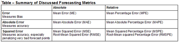
The article has discussed a couple of common error metrics used for evaluating the quality of time-
15 DEC 2016