Sensors - Synchronous Detection - Part III - EdsCave
Main menu
- Home Page
- Sensors
- Simulation
- Analytics
- Forecasting
- Football Forecasting
- Random Corner
- Projects
- Resources
- Blog
- About/Contact
- Creative Works
- Separator 1
- Privacy & Terms
Sensors - Synchronous Detection - Part III
23 May 2016
Some Additional Thoughts....
In Part 1 and Part 2 of this series I wrote about the basic architecture of synchrounous detection and how it works. In this section I will be writing about some things that go into making a practical system.
Phase Compensation.
In the ideal synchrounous detectors previously considered, the only delay was from the output filter -
The demodulated result has double the frequency, but an average value of zero, which is a very different result for the case in which the two sine waves were in phase and the corresponding product would have an average value of 0.5. While this is an extreme case (total loss of output signal!), smaller phase shifts will manifest themselves as system scaling errors. Although one could simply adjust the output scale to compensate, another method is to introduce a parallel phase shift in the carrier reference path (shown below). One advantage of this approach is that it may be possible to replicate the signal path delay in such a way so as to track phase changes resulting from environmental conditions such as temperature. 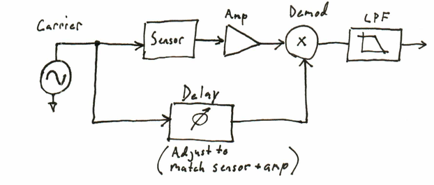
Amplifier Offset Error and 1/F Noise
One big set of system-
Another related issue is 1/F noise. Although an amplifier may advertised as having so many nV/sqrt(Hz) of input noise, this metric can vary as a function of frequency. Typically, as the frequency of interest approaches 0 Hz (DC), the amplifier noise performance gets worse (more noise) in a 1/F manner, with the worst noise density at low frequency. As luck would have it, low frequencies are often where you want to measure sensor signals. While this can be a problem with a DC amplifer/filter arrangement, synchrounous detection systems get around this because they modulate the sensor signal up to the carrier frequency, and tend to reject the 1/F noise from tha amplifier in the same way they reject DC amplifier offset.
Note, however, that the magical rejection of DC offset and 1/F noise only applies to that coming from the amplifier. Offset (bridge imbalances) and low-
Square-
One technique that can greatly simplify the implementation of a synchronous detector is to use square waves for the carrier as opposed sine waves. The first way in which this simplifies the electronics is that it is much simpler to generate a square wave than a sine wave, particularly if you are interested in maintaining precise amplitude and symmetry. The second simplification comes from the nature of the demodulator -

Square-
If the Sensor Signals are Balanced, a DPDT CMOS Switch can Often Serve as a Balanced Demodulator
Because a square-
Spread-
So far this series has mostly been concerned with the problem of rejecting 'random' noise sources that might happen to be in the environment, but have not addressed the problem of dealing with deliberate attempts to interfere with the sensor operation. Injecting an interfering signal at the same frequency and phase of the carrier can be a very effective way of disabling a sensor reliant on synchronous detection. Some security-
While you could use a truly random analog noise source as a carrier, implementing a good one can be a major engineering challenge. Instead, it is typically easier to use what is known as a pseudo-
These techniques are particularly useful in sensor systems which are detecting very small changes in quantity being detected and are highly sensitive to external noise. One example is of capacitive proximity sensors.
Conclusion
Synchronous detection is a powerful technique for implmenting sensor systmes that need high levels of noise immunity or need to recover very small signals. In this 3 part series I have outlined the basic concepts for the technique and described how it operates from both time and frequency domain viewpoints. In the final installment I introduced some variations to the basic technique that can often be used to adapt synchronous detection in real-