Simulation - Block Diagram Notation - EdsCave

5 June 2016

... or,  Differential Equations for Electricians

Ordinary differential equations are one of the the fundamental mathematical structures used to represent continuous time-varying systems.  This does not mean, however, that the mathematical notation commonly used to write them out is the only representation, or even the best representation.  For some problem domains, graphical representations may be better in that they make a system's underlying structure easier to understand and formulate. One popular graphical representation for differential (and algebraic) equations is the Block Diagram.

The use of block diagrams to represent equations has strong roots in several fields of electronic engineering.  The first is control systems, which studies methods of building machines that can behave autonomously. An example of a simple control system would be the thermostat that keeps your kitchen oven at the the desired temperature.  Examples of more complex (far more complex!) can be found in self-driving cars such as the ones made by Google.  Since the 'intelligence' in control systems often used to be realized as analog circuits that were wired out of various components, high-level schematic notations such as block diagrams were developed. This was convenient because the 'blocks' in these diagrams  could then be easily translated into detailed circuit schematics that could then consequently be manufactured into the physical control system.

The second engineering field in which block diagrams were commonly used was analog computing.  Before digital computers became readily available in the 1970's, electronic analog computers were commonly used for engineering computations.  Instead of representing numbers as series of 0's and 1's, analog computers represented them as continuous quantities - for example, the value 3.75 might be represented by a voltage of 3.75 volts on a particular wire in a circuit. Programming an analog computer was performed by connecting various electronic blocks which mimicked mathematical functions with actual wires and a 'patch panel', much as you might wire together various parts of a high-end audiophile stereo system.


Some Functional Blocks

The key feature of block diagrams are functional blocks, which perform mathematical operations.  A functional block has one or more outputs, each of which in turn defines the value for a single variable.  A functional block also may have one or more inputs, which monitor the values of other variables. A functional block with zero inputs is typically used to define either an input variable or a constant, and depending on the chosen notation details may not be explicitly drawn.

The figures below show a few examples of commonly used functional blocks.

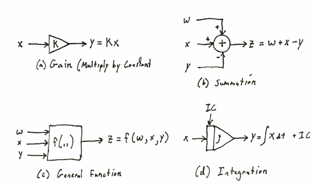
GAIN  (a)  is multiplication by a constant K.  This block defines the output variable Y as being equal to K times the input variable X.  As X is an input variable, it is not influenced in any way, but is simply monitored.

SUMMATION (b) is the addition operator.  In the example shown, Z is defined as the sum of W, X and -Y.  Note the +/- signs at the inputs - this is a simple and unambiguous way of denoting which inputs are to be 'added' and which are to be 'subtracted' (multiplied by -1 before summation) without having to add an additional GAIN block of -1.

GENERAL FUNCTION (c).  A rectangular block is the catch-all for whatever mathematical or logical  function you wish to throw into your system. It can encompass equations, look-up tables, or any other functional form you can devise that transforms the inputs into an output.

INTEGRATION (d).  This block defines integration of the X input variable over time. Note the 'IC' input at the top.  This is used to establish the initial condition for the output variable Y at the start of the simulation (t=0).  Note that integration in this context is implicitly performed over the time variable.



'Wiring' Rules

To formulate a meaningful  or valid block diagram requires that one follows a couple of simple 'wiring rules':

1. Each connected network of 'wires' represents a single variable or constant.

2. All of the inputs of functional blocks must be defined.  This means that you can't leave functional block inputs disconnected, as this would imply an undefined input value.  While some simulation systems may allow this condition by assuming an a disconnected input to default to '0' or some other value, this is a departure from the basic modeling paradigm. After all, what is the value of SQRT(?) ?.

3. The output of a functional block can 'drive' an unlimited number of inputs.  While in house wiring there is a limit to the number of things you can plug into a circuit until you blow a fuse, the wires in a block diagram convey information, and not amperage, so they have unlimited fan-out.

4. You can't connect two or more functional block outputs to a single wire. This is like trying to simultaneously assign two separate values to the same variable - a bit of a conflict.

5. Evaluation 'order'. Whileblock diagram notation is a 'parallel' language in that all functions are continuously evaluated, so there is no intrinsic 'order'.  When you build up networks of functional blocks, however, you do need to understand how they nest.  To continue with the 'computer language' paradigm,  functions further 'upstream' are evaluated with higher precedence, and ones further downstream are evaluated later.  This is where the arrows on the wiring can be helpful.

Keep in mind that the above rules only define what could be called a 'syntactically' valid signal flow diagram. Following them does not guarantee that the block diagram correctly implements your model.


Feedback Loops

Feedback is one of the things that makes for interesting behavior, and is a very common feature even in simple systems.  One downside of feedback is that it can also make for computational complexity. Consider the block diagram shown below.  The two functions F and G are connected in a loop, which represents the algebraic equation shown alongside.  While from a mathematical standpoint, this is a perfectly valid system, it does represent a potential problem from a simulation standpoint.  Assuming that both F and G have well-defined closed-form solutions that allow you to simply plug in input variables and get output variables out, this property may not extend to the system as a whole. If F and G were connected in a way that did not involve feedback as in the figure above, evaluation of the system would be trivial - first evaluate F, then G.

The addition of feedback, however has cast the system into an open-form, where solving for a value of Y requires either symbolic algebraic manipulation or iterative numerical methods, neither of which guarantees a possible solution.  This is a general problem you will encounter whenever you have a feedback loop consisting of 'static' functions, like arithmetic operators, mathematical functions, and anything else where the output changes instantaneously in response to a input change.  For some systems, such as where all of the elements in the loop are linear (e.g. summations and gains) there are well-defined methods for computational evaluation. In most other cases where loops generate non-closed-form algebraic equations, non-linear solution methods are needed, and all bets are off.  From a practical standpoint, this situation is typically handled in one of two ways. The first, is when your simulation tool recognizes static loops and  applies various numerical methods in an attempt to find approximate solutions. The second method is when the tool recognizes the loop it will simply report it back to you as error.  In general, static loops should be avoided if possible both for the computational issues that come with them and because their presence is a hint that you might need to re-think your model formulation - at least for a block diagram paradigm.

Although static loops can be problematic, loops that are broken up by integration blocks, such as can be seen in the figure below,  are not, and such loops are extremely common in the kinds of systems typically represented by block diagrams.  While you still end up with non-closed-form equations, their numerical evaluation becomes straightforward.  The process of numerical integration essentially breaks the feedback loop at the integration blocks.  Since numerical integration assumes that the integrator output is held constant from one simulation time 'tick' to just before the next tick, it can be treated as is it were a constant input into the system, and only re-evaluated when the simulation clock advances.

An Example

We will now consider a simple example of how one gets from physical system to a block diagram model.  The key element of the system to be considered is a mass 'M' that has been mounted on ideal frictionless wheels so it can roll back and forth (figure below). Attached to the left side of this mass is a spring so that the mass will tend to be constrained around a horizontal position of X = 0 (horizontal displacement).  Since we are assuming an ideal frictionless system, as generations of idealistic physics students have, if we were to pull the mass to the left and let it go, it would oscillate back and forth forever.

To make the system a little more realistic, we will add some damping with a device called a dashpot, connected to the right-hand side of the mass. The purpose of the dashpot is to damp out the oscillation over time, by providing a force that opposes any horizontal motion. Unlike a spring, the force contributed by the dashpot is independent of the position, but is proportional to the speed of motion.  Dashpots, by the way, are real devices that you can actually buy - they were not conjured up by physics professors for toy problems.

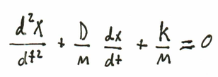
Each of the elements of the simulation has various properties such as forces, velocities, positions and accelerations, which all vary as a function of time.  The following list shows the key relationships:

a) The spring force Fs is proportional (by 'K', the spring constant) and in opposition to the position (X) of the mass M.
b) The damping force Fd is proportional (bt 'D' the damping constant) and opposes the velocity (V) of the mass M.
c) The acceleration of the mass (second derivative of position) is controlled by the sum of the forces acting on it, and inversely proportional to the mass M. If you have a bigger mass, it accelerates more slowly (F=mA).
d)  Velocity (V) is the integral of acceleration over time.
e) Position (X) of the mass is the integral of velocity over time.

All of the above could be combined to form the following ordinary differential equation (shown below), which could then be solved for position X as a function of time through well known methods that would require finding my old differential equations textbook.

Since the purpose of this post is to discuss signal flow graph models, my differential equations book shall remain entombed in a box in my basement. Instead, let us consider how the above equations map into the block diagram shown below:

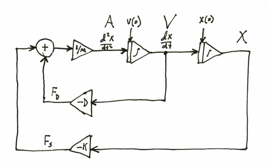
The integral relations in equations (d) and (e)  are realized by the two integation blocks placed in series, which sucesisvely transform acceleration into velocity and finally into position. The forces from the spring (eqn. a) and dashpot (eqn. b) are developed through gain blocks respectively driven from the X and V integrator outputs. Finally, these are converted back into acceleration by summation and being multiplied by 1/M (eqn. c).

While the choice of functional blocks and the connections between them are dictated by the physical system's mathematical model, there is a certain art to drawing a block diagram so that the system's structure is apparent.For example, in this system, one can clearly see the feedback relations between velocity and position and the acceleration. This is one of the major strengths of block diagram representations - when properly rendered they allow you to quickly see system relations that might not be as apparent when looking at a set of equations.


System Behavior

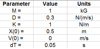
If a block diagram contains no static feedback loops, it can be straightforward to simulate. For a system as simple as the one presented above, an effective simulation can even be realized using a spreadsheet.  As a check, lets implement the model, and assign the following parameter and initial values:

In the resulting plots shown below, you can see three effects which you would intuitively expect from this type of system:

1) The cart bounces back and forth sinusoidally (spring and mass action)
2) The bouncing dies out (the action of the dashpot)
3) Velocity and acceleration are 90 degrees out of phase (two sinusoids related by integration or differentiation)

Note that the solution shown above is from a step-by-step (time steps every 0.05s)  numerical integration of the system - not by the analytic solution of the differential equations.  The strength of the simulation approach is that it can handle much more complex systems than this one, while analytic methods can become very unwieldy very quickly.

To conclude, block diagram notation offers a powerful way of describing complex dyanamic systems. The graphic nature of the representation often reveals system structure that might not be apparent when looking at traditional equation-form descriptions of the system. Block diagram notation also has the advantage that it can be translated into executable simulations very easily, both manually and by automated tools.