Forecasting - Exponential Smoothing - EdsCave

19 July 2017

In a previous article, we discussed the use of simple and moving averages as a way to forecast the future values of stationary processes.  While simple averaging of all prior data samples yielded an optimal estimate for the next unknown samples, it suffered from the drawback of slow response to changing conditions – when the data series was not truly stationary, but experienced either sudden shifts or slow drift in its underlying statistics.  To handle these cases, we introduced the concept of the moving average, which only considers a set number of prior samples, effectively ignoring data points in the distant past.

       (eqn. 1)
K-point moving average   

The primary reason for using the moving average is the idea that older samples (outside the averaging window) carry less information relevant to developing a forecast, and can be ignored.   Samples within the window, however, are given equal consideration regardless of age.   If you want to give some samples more of a 'vote' than others, it is straightforward to add a 'weights' to the samples within the average. This might be useful, for instance, in the case where you want to give the more recent samples more influence than the oldest ones.  A weighted average can be defined by the following equation, where the 'a i ' terms are the weights:

(eqn. 2)

In the above expression, you must ensure that all 'a[i] ' terms are positive and that their  sum equals 1.  An alternate version of the above expression that relaxes the requirement that the weights add up to 1 is:

(eqn. 3)

Implementing a weighted moving average in a spreadsheet is a bit more complex than implementing the simple moving average. One way of doing so is to define a column with the weight values and use the SUMPRODUCT() and SUM() functions to implement the above equation, as shown below:

The next question that may come to mind is that of how we go about picking weight values? In the above example, we just arbitrarily chose weights of '1', '2' ,' 3'  and '4', with '4' being applied to the most recent sample.  Finding a good set of weights to use (never mind finding an 'optimal' set) for a given application and data set  can be a complex problem, compounding the already difficult question of how many samples to use.   The main issue is that for a k-point weighted moving average, you have 'k' decisions to make in choosing weights.

One common approach to the 'weight selection' problem is to select a rule that defines the weights.  For example, the rule for the moving average is 'use all equal weights'.  Selecting a weighting rule reduces the number of decisions you must make. Even more importantly, selecting a rule that has been extensively used before  also has the advantage that its properties may be well understood.

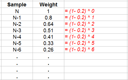
One common rule is 'exponential weighting', which assigns higher values to the most recent sample and possessively lower weights to older samples. The reason that it is called 'exponential' is that the weights drop off exponentially by a given decay factor  α, where weights are determined by (1- α) ^ N , where greater N implies weights further back in time.  For example, a weighting based on α = 0.2 is shown below.  

Even when using a  an exponentially weighted moving average, we still have three issues to consider:

1) What value of α should be used?  Note that to get an exponentially decaying weight,   α must be between 0 and 1 ( 0 <  α < 1) .
2) How many samples (k) should be used?
3) Handing 'start-up' predictions where fewer than k samples worth of input data are available.

The first and second issues are inter-related, as a larger decay factor and larger number of samples allow for a greater rejection of random noise in the input data, but trade this off against slower and reduced  response to more significant changes in the input data. As we have seen in the last article, one way of dealing with the third issue is to simply refuse to make predictions until you have enough data points to correctly perform the moving average. The other approach is to start-up your early forecasts based on averages with fewer than the prescribed number of points. While this is relatively easy to do in the case where the weights are uniform, it gets a bit more complex to decide how to handle this properly when the weights have differing values.

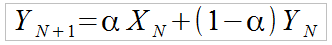
One neat property of exponential weighting is that there is a very simple and elegant implementation that solves problems #2 and #3 above.  We can define the next forecast data point (Y[N+1] ) in terms of the present input value (X[N ]) and the previous forecast value (Y[N] ) as follows:

(eqn. 4)

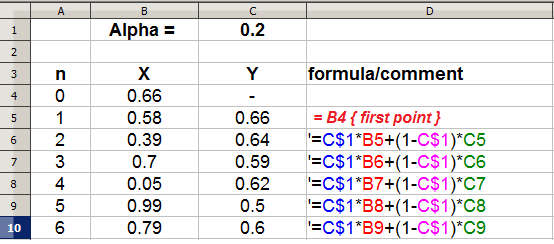
Let's see how this can be implemented on a spreadsheet:

So how do we get exponential weighting out of the above formula (eqn. 4)? If we walk through a couple of steps and expand the formula out in terms of just the inputs (X's), we get:

(eqn. 5)

After some algebra, a pattern emerges – successively older values of X end up being multiplied by increasingly higher powers of (1-α ) - and as long as 0 <  α < 1, this gives us exponentially decreasing weights.

Some of the features of this method, commonly called exponential smoothing are:

1) The forecast incorporates some information from every prior point. The further back the data point, however, the less weight is assigned.
2) Except for the first forecast (Y1 = X0), the method  requires no special attention to 'startup'
3) The method properly handles the scaling of the weights through the α and (1-α ) terms.
4) Because the X[0]  term is just multiplied by (1- α) k , as opposed to  α(1- α) k  like the other X terms, it will have a pronounced effect on the forecast for quite a few cycles – at least until it falls far enough back into the past for (1- α) k  to become small in relation to  α.
5) The only parameter you need to choose is  α.

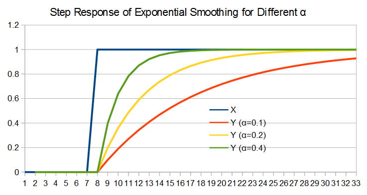
The last of these features, choice of α makes exponential smoothing relatively easy to use. The big question, though, is how to choose  α?  In general, lower values of  α make the forecasting function less responsive to changes in the input data (X) , but reduces the effects of noise. Conversely,  higher values of  α result in quicker responses to changing input data, but also pass more noise through to the output. An example of how some different values of  α behave is shown in the figure below.

Another way of thinking about the effect of  α is the step response of the exponential smoothing process. Instead of using 'real' data for the input, we use a step function – an input data set that starts out with a value of '0', and then at some point transitions to a value of '1'.  This type of input data set makes it very clear how fast the exponential smoothing function reacts to changes, as can be seen in the figure below.

Note that since we are defining a one-step-ahead forecast, (Y[k+1]), there is a single step delay between the input change (X) and when the output begins changing.  An important feature of above plots is how long it takes the output (Y) to cross the 63% mark once the input changes – this is known as the time constant of the smoothing function, and it is given by ~1/α (more accurately as α gets smaller).  Features in the input data that are of much shorter duration than the time constant (such as noise and single-sample 'glitches') tend to be smoothed out, while features of much longer duration tend to be passed along.

The above described ability of exponential smoothing to remove spurious noise from data is more commonly used as a filter than as a forecasting method. Similarly, moving average and weighted moving average operators are also used more commonly for filtering than  forecasting.  In cases where the process generating the data is more or less stationary, however, filtering the data can be an effective way of forecasting – at least when a forecast value for the very near future is needed.