Forecasting - The Moving Average - EdsCave

The Moving Average as a Forecasting Method

In some situations, forecasting need not be complex at all. In this chapter, we will look at the use of the average (arithmetic mean) and moving average for predicting future values of a time series.

To effectively use averaging as a forecasting tool requires that the process being forecast has neither trends nor periodicity.  One type of process that meets these requirements is simply a time series of constant values ( 'a' ) .  Forecasting this kind of process, however, tends to the trivial. A related, but  more interesting type of process is one in which that unknown constant value  is combined with random fluctuations.  

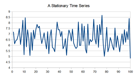
Consider the time series in the graph below.  By casual observation, it can be seen that there is no clear upwards or downwards trend, and that while there may seem to be some stretches that look like they might represent periodic behavior, these stretches do not persist for very long. Individual values range from approximately 5 to 8.5, with a central tendency somewhere around 6.5 or 7. Seeing that the last observed value is approximately 5,  what might be a likely candidate for the next (unseen) value?

If one assumes that the process generating the above time series can be modeled as a constant with added noise,  the prediction challenge hinges on whether the noise remains consistent over time – and this can be seen in terms of its statistical distribution. Since we don't know the underlying process that generated this time series (well, I do – but you don't!), a first test might be to look at the distributions and statistics for different parts of the time series.  The figure below overlays histograms for the first and second half of the above data (50 points each).

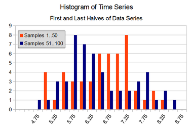
The distributions from the two halves of the time series do seem to have considerable overlap, but with only 50 points each, it is difficult to say that they are clearly equivalent or clearly different.  If we consider the means and standard deviations of the two samples, they are credibly close.

A process whose output has a statistical distribution that doesn't vary over time is called stationary. Note that the output values may vary over time – it is the distribution of those values that doesn't. The result is that if you take a large enough samples of output values over two separate intervals, their distributions should be identical.  In the example above, the two 50 sample sets are enough data points enough to suggest the generating process is stationary, but not absolutely clear.  In addition to the 'eyeball test', more quantitative methods such as Student's T-test can also be used to determine the likelihood that two samples are from the same distribution.

You may also notice that the two distributions are roughly 'normal' – that is they can be described (albeit very approximately) by a bell curve.  If we assume that the process generating this data is both (a) stationary, and (b) normally distributed, then the optimal estimator for this process is simply the average of all prior values.  This means that the best estimate for the unknown sample #101 is ~6.62 (the average of all prior samples), and not closer to 4.83 (the value of sample #100).  

How well does the average work as a predictor? As an example, consider the chart below, which displays a stationary time series, and the cumulative Mean Absolute errors (MAE) for predictions made by both the running average forecast and the naive forecast (the next sample will be the same as the present one).  The 'average' forecast has about 25% better accuracy than the naive forecast, and using more sophisticated forecasting methods would make no improvement (in this example) because the process being forecast is both stationary and normally distributed.  

So if the simple cumulative average is the optimal method of forecasting the next value for a normal, stationary system, why would we need any other methods?   


The Moving Average

Before tackling the question of why we might need to concern ourselves with any other forecasting techniques for stationary sarees when simple averaging is optimal, let's first take a look at what is a moving average.

To perform a moving average simply means that one takes the average of some number ('N') of immediately prior data points in a time series, as opposed to taking the average of all prior points.  The spreadsheet below provides an example of a three-point moving average (N=3):

In this case, column B (Y) is the data we want to average, and column C is the result. The formulas used in column C are shown for reference in column D.  In this case we are taking a 3-point moving average, where each cell's value in the C column is the average of the corresponding and two 'prior' cells in the B column.

In the general case, for an 'N' point moving average, each averaged data point   'M[k]'  of data series 'Y' is defined as:

M[k] = Average( Y[k+1-N] … Y[k])

One issue with moving average methods that is shown in the above example is that of 'startup' – or how do we calculate  meaningful moving average values for the initial cases where we have fewer then 'N' input data points. Two common approaches are:

• Leave them blank (as we did in the above example)
  

• Take lower-N moving averages. In the above example, C2 could be set to AVERAGE(B2)  (N=1), and C3 could be set to AVERAGE(B2:B3) (N=2). Doing this means that these initial points do not obtain the full benefit (or any benefit in the case of C2) of the moving average process.  The value of having these initial points, however, often outweighs their lack of averaging.
  

So now that we know what a moving average is, how might it be applied to the forecasting problem. And why might we prefer using it to the 'optimal' simple average?

While the simple average may be optimal for forecasting the next point in a stationary, normally distributed time series, it may not remain optimal if either of these conditions is violated.  One very common violation occurs when the series does not remain stationary, and its statistics shift over time. Consider the case of the time series shown below, where the mean abruptly changes.

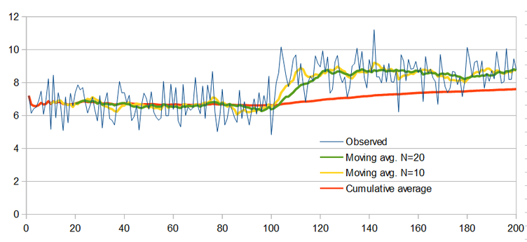
In this example, it can readily be seen that the mean value of the observed data shifts significantly upwards around sample 100.  The simple average (orange), tracks this change only very slowly, so that even by the 200 th  sample, the average has only made it about halfway to the new mean value around which the observed data has settled. This is because the simple average equally weights the entire history of the time series, even very old points that may no longer be especially relevant to the present conditions. On the other hand, the moving average ignores old data past a certain point.  The yellow line shows the result of a 10-point moving average, while the green line shows that of a 20-point one. Note that both moving averages settle in to track the time series much more quickly than the sample average does, as the moving averages ignore older and irrelevant data points.

When using a moving average, one big question is that of how many points ((N) to use. The above example shows the results for both 10 and 20 point moving averages . While the 10-point moving average responds more quickly to changes in observed data than the 20-point one, it also is more susceptible to short-term noise.  Balancing responsiveness to time series changes against the ability to average out noise is a key tradeoff that needs to be made when selecting the number of points to use for a moving average.

The key value of the moving average is that it can be effective at forecasting time series which may appear 'stationary' in the short term, yet are not when observed over a much longer time frame. The above example used the case of a time series with an abrupt shift in statistics, which can happen when a system is subject to shocks or discontinuities. For example, if a product is newly added to or removed from the sales offering of a chain of stores,   that product's  average sales are likely to increase or decrease in discrete jumps, with the timing corresponding to the  when the product was introduced or retracted.  

Changes to the system being forecast need not occur as a result of discrete events. Another common situation is where the system has clear long-term continuous variability, but in the short term is relatively stable and and 'stationary'.  An example is outdoor temperature.  Where I live, the average temperature for January is ~30F, while the average for July is ~75F.  When predicting a daily average, using a moving average filter with a relatively low value of 'N' (~10-20 days?) will tend to give a much better forecast than simply using the long term (annual) average temperature of ~50F.  Of course,  there are better ways of predicting the weather than by using moving averages, but this case shows an very clear example of a system that is non-stationary when observed on one timescale, but appears more stationary on another, shorter timescale.