Simulation - A Vibrating String Model - EdsCave

3 JAN 2016

This blog will discuss a physical simulation of system that all you musicians out there should be familiar with - a vibrating string.

Familiar example of vibrating strings

The physical system is pretty simple to implement in the real world. You take a string or a wire, and you attach it to two endpoints, and apply some tension. This is the basis of 'stringed' instruments such as the guitar, piano and violin.

An ideal string in 'Flatland' - it can only move in the 'Y' direction

Strings on real instruments can behave in many 'interesting' ways, depending on non-ideal properties and behaviors - this is the basis of lots of interesting musical effects, and a few annoying ones, such as when the density becomes non-uniform and the string goes 'false' - a real problem for violinists.  For this simulation study we are going to assume a very 'ideal' string:

1) The density (mass/length) is uniform.
2) The elasticity is perfectly linear.
3) There is no friction or other losses - it will keep vibrating forever.
3) The only motion is in the 'Y'  direction in an X,Y plane - no Z or X motion is allowed.

The mathematical relation that describes this system is well known, and is called a Hyperbolic Partial Differential Equation. If you say it out loud this sounds really cool, like something you use for programming the warp drives on the starship Enterprise. But it is also known as the 'wave equation', as it and related forms describe the propagation of all kinds of waves, both acoustic and electromagnetic.

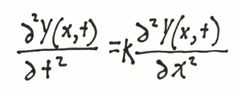
A Hyperbolic Partial Differential Equation looks as cool as it sounds

So what does this equation mean?  Translated into English, it says that the second derivative of the 'Y' motion with respect to time (the left side)  for each point along the string is equal to the second derivative of 'Y' with respect to 'X'  (the right side) for that point. For this physical system, these two derivatives have intuitively understandbale equivalents - the left side represents the up or down acceleration of each point on the string, and the right side represents the curvature of the string.  The constant 'K' is a function of both the tension on the string and the density per unit length.

For a numerical simulation, we model a String as a series of discrete points.

Although this type of  hyperbolic PDE has an analytic solutions, we are interested in a numerical simulation. The first step in doing this is to approximate the continuous problme by a discrete one, where the string is modeled as a series of points along it. The spacing between points in the 'X' direction will be called Δx. The solution we will come up with will only descibe the positions of these discrete points. If for some reason we were to care about points in between theese points, these could be estimated by interpolation.  In a discrete simulation, it is important to have anough points to be able to accurately describe the expected phenomenon.  For example, if we were interested in modeling a standing wave with 4 periods (shown as an example below), we will need a lot more than 4 points to model this properly - for example, 50 or 100 might not be a bad place to start.

Curvature (2nd derivative in X) controls how each point is pulled up or down

When breaking the string up into a series of points, it becomes intuitively obvious how the curvature, or second derivative relates to the acceleration. If you consider three points along the string assume the outside ones are fixed, that the central one is free to move, and pretend they are connected by elastic segments, there are three possible behaviors. The first case is when the curvature is negative, the stretched segments will try to pull the middle point down (negative acceleration). The seocnd is when the middle point is lower than the outer ones, in which case the stretched segments will try to pull the middle point up (positive acceleration). The final case is when all points are in a line, and the middle point is pulled both up and down equally, and as a result experiences no overall acceleration.  

Once we have modeled the string as a series of points spaced by Δx we then have to come up with a discrete approximation to the second derivative.  When learning calculus, the first derivative is usually described as (y(x+Δx) - y(x))/Δx, where Δx approaches zero.  In the case of numerical soluations, we don't let Δx approach zero, just some arbitrarily small, but still finite value. Without going through the complete derivation, it is possible to model the second derivative of Y with respect to x for a single point as shown below. By pluging some numbers into the sub-expressions for 'left point', 'middle point' and 'right point' one can perform some quick sanity checks that this approximation does indeed provide a measure of the 'curvature' of the three points.

A discretized approximation for the second derivative with respect to 'X'

Similarly, we can also approximate the second derivative with respect to time the same way, as shown below.  This may seem a bit strange at first glance, as this expression involves knowing a future value of Y, specifically the subexpression Y(x,t+Δt).

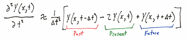
A discretized approximation for the second derivative with respect to time

Having a future value for Y somewhere in the expression is actually very important, at it allows us to form an explicit equation defniing that future value in terms of previous values. If you set the above two apporximations equal to each other (as they are in the PDE), and solve for Y(x,t+Δt), you get the following expression:

Combining the previous two equations provides an explicit 'update formula' to compute Y(x, t+Δt) - the position at the next timestep

The following figure shows one way of visualizing the relationships between points in time and space. The top point is the future value of Y at a given point, yet to be computed. The points in the row below represent known current values for that point and its immediate neighbors, while the point at the bottom is the prior value of Y.  Knowledge of that previous point is essential to computing the second derivative in time.

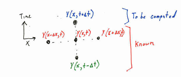
Graphic relation of points in expression - vertical axis is Time, horizontal axis is 'X'

After all of the above theory, it turns out that the 'computer' part of the computer simulation is pretty simple. Below is some example code for performing the update step - or the calculation that computes the next values of all of the Y points at time t+Δt). To 'run' the simulation, you need to set the iniital conditions (Y() and Y1() arrays) and wrap the code below in a loop that steps through time by timestep Δt.  Note that this simulation 'kernel' requires only 7 lines of code!

 // Y()   - global is the vertical displacement of each point in the string.
 // Y1()   - global is the previous value of Y.
 // Ynew() - temporary to hold next timesteps.
 // NPts is the upperbound in the Y and Y1 state arrays
 // dx = 1/NPts - the length between points
 // dt is the timestep
 // K is a scaling constant that accounts for the tension and mass of the
 //      string (tension/mass).
 // Only update points 1..N-1, points 0 and N are fixed endpoint boundaries

 // Calculate new position
 for i = 1 to Npts-1
    Ynew(i) = 2*Y(i) - Y1(i) + K *((dt*dt)/(dx*dx)) _
              * (Y(i-1) - 2*Y(i) + Y(i+1))
 next
 
 // Update prior and current position
 for i = 1 to Npts-1
   Y1(i) = Y(i)
   Y(i) = Ynew(i)
 next
 
Of course, more than half the fun of a simulation is how it responds to different inputs - and this requires considerably more than 7 lines of code to read input parameters, set up initial conditions, and provide a graphic animation to watch.  The implementation of these details will be left as an exercise for the student ;).  

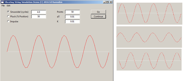
So how does our vibrating string model behave?  If we set an initial condition of 4 cycles of a sine wave, the lobes bounce alternately positive and negative in what is known as a standing wave pattern. This behavior is exactly what we would expect from a physics-101 explanation of waves, and is also one of the easiest-to-derive anlytic models for this system.

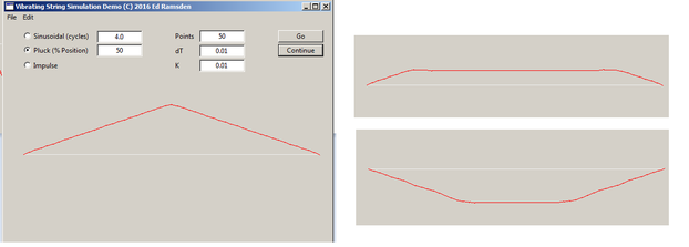
The real value of numerical simulation is that it allows us to look at cases that are more complex than the typical textbook ones. for example, consider the case in which the string is held at a single point in the center, and then released [1].  This has a very different behavior in that a region of flatness spreads out as the string moves toward the center position and reforms as a triangle on the negative side before reversing direction.

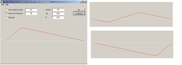
If you pluck the string at some point other than the center, the wave appears to move to the right and bounces off the end in reversed polarity. This wave reflection phenomenon is also something you would expect from a physics-101 knownledge of waves.

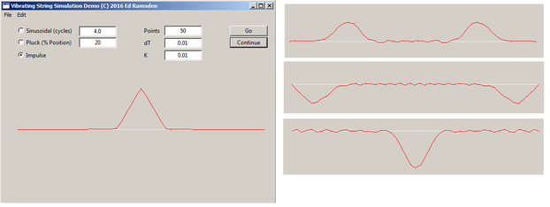
A much better illustration of the reflection phenomenon can be seen if the initial condition is a single pulse in the middle of the string - although setting this initial condition in reality could be a challenge!  In this case, the single pulse splits into two which head off in opposite directions along the string,  reflect with negative polarity off the ends, and then pass through each other, briefly appearing to recombine into a single negative pulse along the way.

If you looked at the above examples closely, one thing you may have noticed is that 'dT' is a very small value. This has two effects. First it makes the simulation run slower, as it traverses less time with each 'update' cycle. More importantly, it maintains stability. Like other simulations in which there are feedfback loops present, not only will the accuracy suffer with too large timesteps, but the solution will very quickly numerically explode into something meaningless, as in the following example with dT set to 0.3:

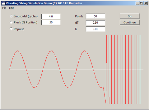
Too big a time step results not only in poor accuracy, but sometimes even numerical instability (shown)

Notes:

[1] - Actually, the plucked string analytic solution is not all that complex, but the solution is an infinite series.

References:

Partial Differential equations for Scientists and Engineers, Stanley J. Farlow, Dover Publications 1993, New York